Introduction
tldr; Getting the most out of your hardware matters a lot in modern ML. There are plenty of tools for this. In this post we use Nsight Systems to profile and optimize the GPU utilization of a real training pipeline.
A lot of ideas in modern machine learning are older than they look. Many date back 40 or 50 years. What changed is that hardware finally caught up and made it possible to actually run them. It really does make a difference whether your training epoch takes 1 second or 1 hour. Obvious in hindsight, but the same observation still holds today, even with Moore’s law having had 50 years to do its thing.
Instead of working through toy examples, we’ll profile a real production codebase. Partly because I have to optimize its performance anyway, and partly because toy examples mostly teach you how to solve toy examples. We want to learn the workflow.
Installation
You need nsys installed on both the machine doing the work (a remote GCP instance in my case) and your local machine with a GUI (my laptop). The versions need to be compatible. Your local machine doesn’t need an NVIDIA GPU or drivers. Download it here. For installation details, just ask Claude, it genuinely knows more about this than I do.
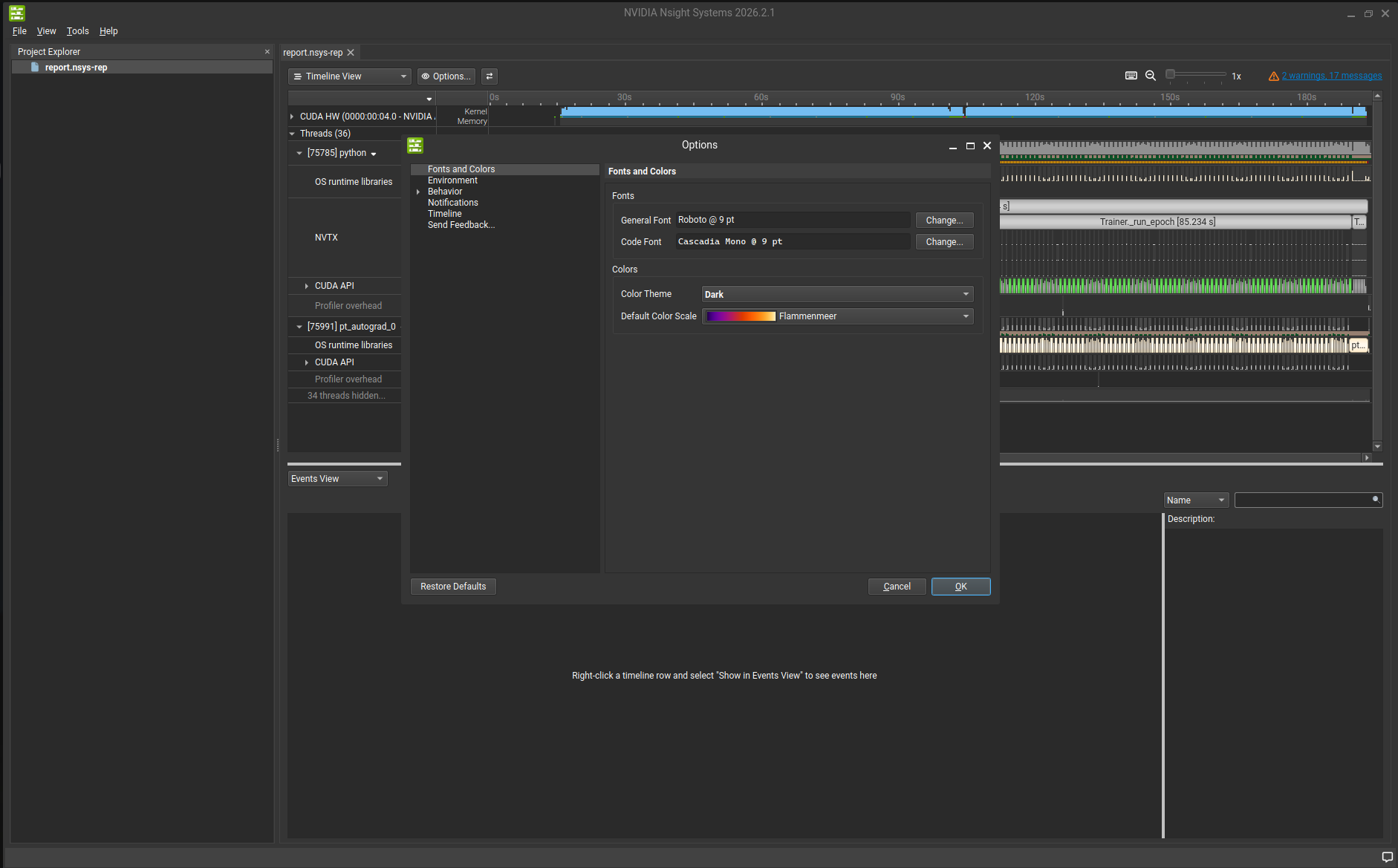
Heads up: If you open Nsight Systems for the first time, it will flashbang you. Switch to dark mode at
Tools > Options > Color Theme.
Profiling your first program
Here’s how profiling with nsys works. Assume you have a training script you’d normally run like this:
python train.py --config configs/default.yaml
Assuming you have nsys installed, you can just prepend the profiling command:
nsys profile \
  --python-sampling=true \
  --backtrace=none \
  --trace=cuda,nvtx,osrt \
  -o profiling/report \
  --force-overwrite true \
  python train.py --config configs/default.yaml
You don’t need most of those flags, but here’s what they actually do:
--python-sampling=true: nsys periodically samples the Python call stack of your running program. This lets you hover over any point on the timeline and see exactly what Python code was executing at that moment.--backtrace=none: Disables C++ stack unwinding for CPU events. This cuts profiling overhead significantly without losing much useful information for most use cases.--trace=cuda,nvtx,osrt: Tells nsys what to record.cudacaptures all GPU API calls,nvtxcaptures any custom range annotations you add to your code (more on that below),osrtcaptures OS-level events like thread synchronization.-o profiling/report: Path for the output file.--force-overwrite true: Overwrites an existing report rather than erroring out.
Once the run finishes, download the .nsys-rep file to your local machine and open it. You don’t need an NVIDIA GPU locally, but you do need a GUI:
nsys-ui report.nsys-rep
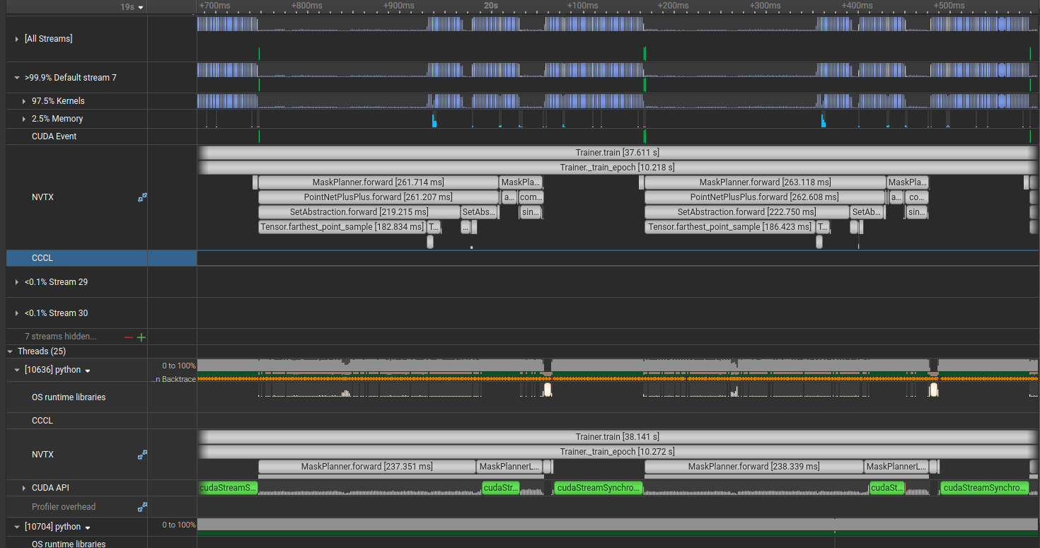
This opens something like this:
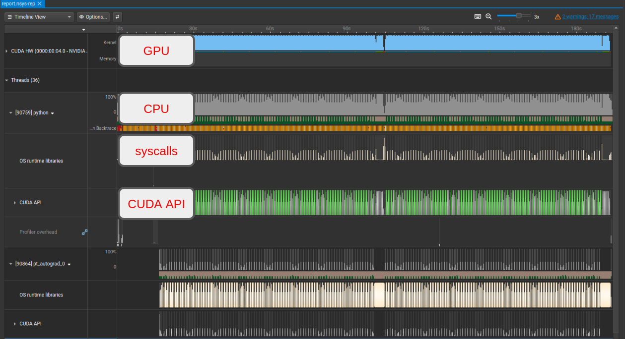
Navigating the UI: left-click drag to select a region and press shift+z to zoom in. backspace undoes the zoom. Hovering over most things shows an info overlay.
The top row is your GPU. It shows SM utilization (how much compute you’re using) and memory utilization. Since the GPU is almost certainly the most expensive component in the system, you want both of these high. SM utilization in particular should stay high as continuously as possible. Below that you see the CPU threads. The thread labeled [90759] python is the main thread and is almost always the one to watch. The others are usually background workers you can mostly ignore. If you’re curious what they’re doing, click the + in the bottom left to expand hidden threads.
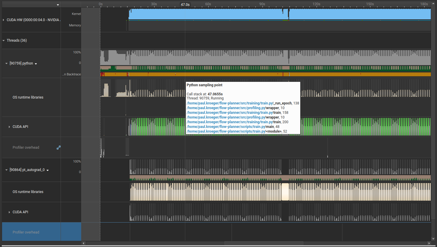
The --python-sampling=true flag means nsys captures call stacks at regular intervals. Hovering over one of those timestamps shows what Python code was running at that moment, which turns out to be very useful for tracking down unnecessary synchronization points.
Below the CPU threads you’ll find system calls (what your program asks the OS to do, useful for understanding when data is loading) and the CUDA API row. We’ll spend a lot of time looking at the CUDA API row. GPU syncs show up in green, and you can spot when the GPU is allocating memory here too.
Ok, now let’s make things go brrrr.
NVTX annotations
Nsight Systems doesn’t require you to modify your code, which is nice. But adding annotations makes it much easier to understand what you’re looking at. Specifically, we want NVTX ranges. These let you label sections of your code so they show up as named regions in the timeline.
I use this boilerplate, adapted from this post:
import contextlib
import torch
import functools

def nvtx_annotate(fn):
    @functools.wraps(fn)
    def wrapper(self, *args, **kwargs):
        with nvtx_range(f"{self.__class__.__name__}.{fn.__name__}"):
            return fn(self, *args, **kwargs)
    return wrapper

@contextlib.contextmanager
def nvtx_range(msg: str):
    depth = torch.cuda.nvtx.range_push(msg)
    try:
        yield depth
    finally:
        torch.cuda.nvtx.range_pop()
I usually put this in src/profiling.py and import it wherever needed. nvtx_range works anywhere. nvtx_annotate is a decorator for class methods specifically.
One thing to keep in mind: NVTX ranges on the CPU and GPU don’t necessarily line up in time, and that’s expected. The CPU submits work to the GPU via a command queue asynchronously, so an NVTX range pushed on the host side will often start well before the GPU actually begins executing that work. Both timelines are accurate, they’re just showing you different things.
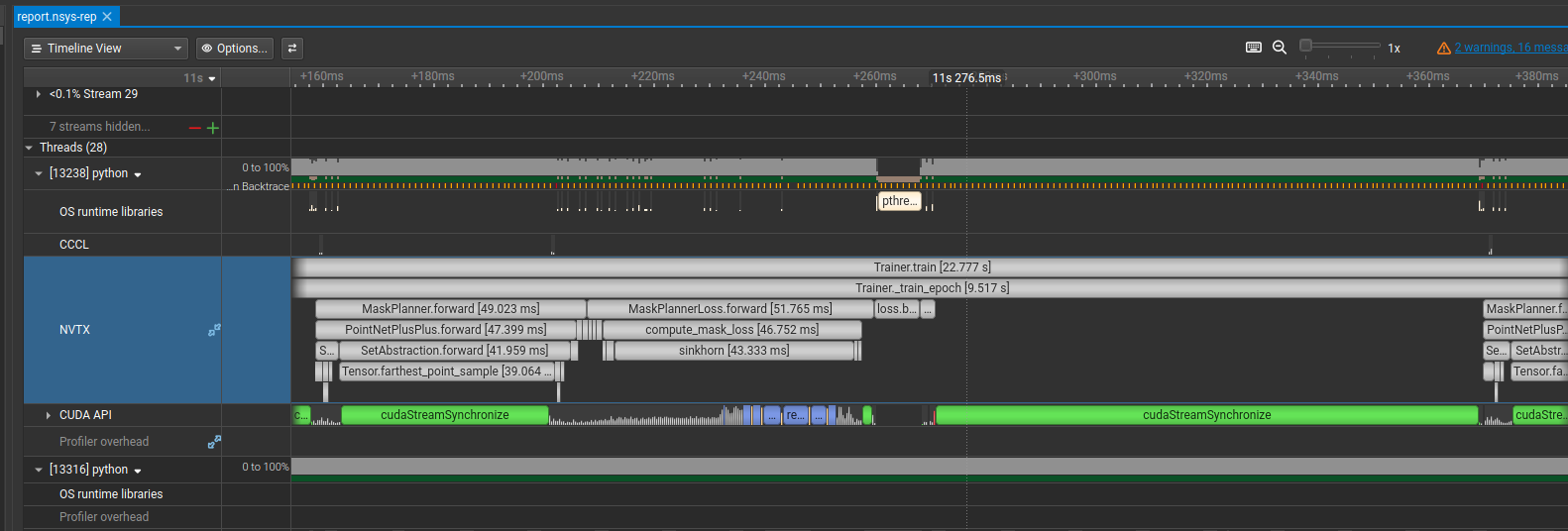
After sprinkling annotations through the relevant parts of the code, the profile looks like this. The important thing is that annotations should cover essentially the whole execution. If there are large unlabeled gaps, you have sections doing significant work that you can’t see or optimize.
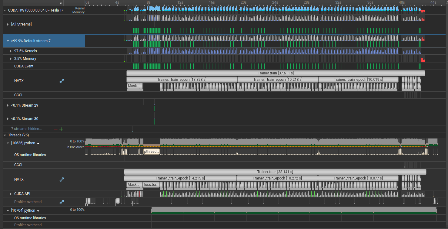
You’ll notice GPU utilization is pretty spiky. There’s a lot of room to improve here. I’ve seen a similar picture in most research codebases I’ve worked with.
When zooming in, start from the middle of the trace rather than the beginning. The start of a run is noisy with initialization, and once things are warmed up you get a cleaner view of steady-state behavior.
Actually, wait. We almost forgot the most important thing: we need a metric to track. Otherwise we’re just vibing. Throughput in samples per second is a good choice because it naturally accounts for batch size and dataset size:
t0 = time.perf_counter()
train_loss, train_breakdown, n_samples = self._train_epoch(epoch)
torch.cuda.synchronize()  # make sure all GPU work is done before stopping the clock
epoch_time = time.perf_counter() - t0
throughput = n_samples / epoch_time
The torch.cuda.synchronize() call is important here. Without it, you might stop the timer before the GPU has actually finished, which would make your numbers look great for completely wrong reasons.
Our starting point is around 65 samples/second.
DataLoader
Data loading is one of the most common bottlenecks. It can easily happen that the GPU sits idle waiting for the next batch. PyTorch gives you a few simple levers:
- Increase
num_workersin your DataLoader - Set
pin_memory=True - Use
.to(device, non_blocking=True)when moving tensors to the GPU
These three changes took about 5 minutes and brought throughput from 65 to 75 samples/second. Decent for essentially no work.
Use library functions when they exist
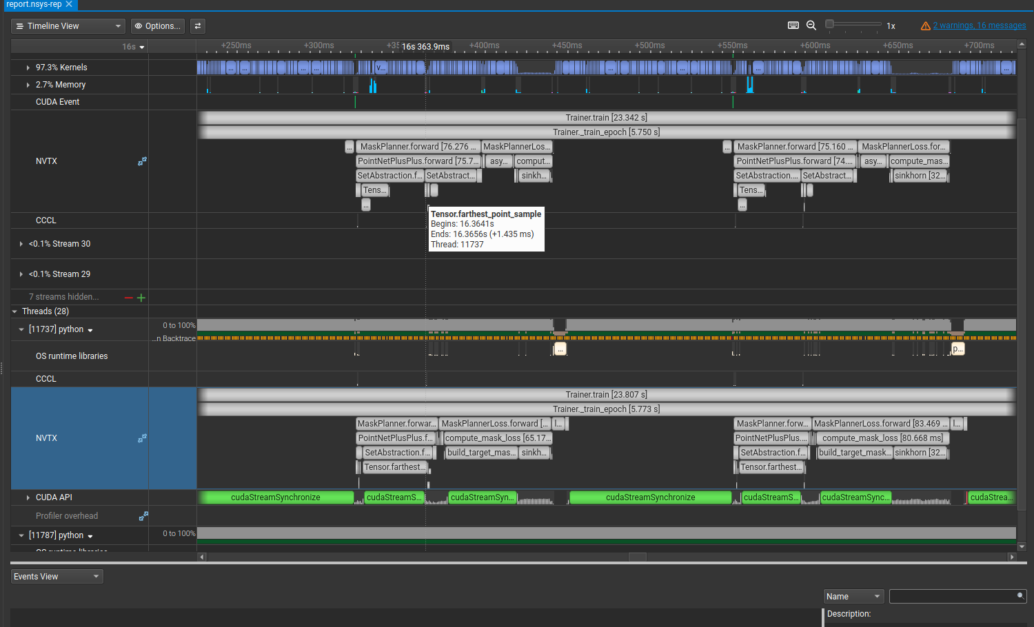
Zooming into the forward pass, there’s a section where the GPU goes completely idle for 187ms. The NVTX annotation labels it as Tensor.farthest_point_sample.
Looking at the corresponding code reveals a custom farthest point sampling implementation. Nothing wrong with it per se, but torch_cluster ships an optimized FPS implementation. Let’s try swapping it in.
We go from 75 to 140 samples/second. Almost 2x, by installing a package and replacing 10 lines of code.
Why didn’t the original code use torch_cluster? My guess is that the author either wanted to avoid the dependency, didn’t know torch_cluster had an FPS implementation, or an LLM wrote the code and made the same call. I’ve seen this pattern more than a few times. If something looks like a standard geometric or graph operation and it’s showing up as a major bottleneck, it’s worth checking whether a library already has an optimized implementation before spending time on a custom one.
You really don’t want to sync your GPU
Time to talk about synchronization.
Here’s the simplified version of the CUDA compute model. When your CPU encounters a heavy computation, instead of doing it inline, it submits a kernel to a GPU command queue and immediately moves on. The GPU picks up that kernel and executes it asynchronously. The CPU doesn’t wait around because the hope is it won’t need the result right away and can get other work done in the meantime.
At some point the CPU does need the result. That’s when it has to sync with the GPU, meaning it stalls until all queued GPU work has finished and the results are available.
The issue isn’t that syncing is inherently bad. You always have to sync somewhere. The problem is that an early sync punctures the pipeline. The GPU’s scheduler is good at keeping work queued up and hiding latency by pipelining kernels. A sync collapses that: the CPU stalls, stops submitting new work, and the GPU drains its queue and goes idle waiting for the CPU to catch up and give it something to do. Instead of overlapping CPU and GPU work, you’re paying the full round-trip latency at that point in the program.
The tricky part is that syncs don’t always come from obvious places. Functions you think of as utility code, things you’d happily hand off to an agent to implement, can quietly contain a cudaStreamSynchronize that brings everything to a halt. A large green block in the CUDA API row for a function like build_target_masks is a red flag.
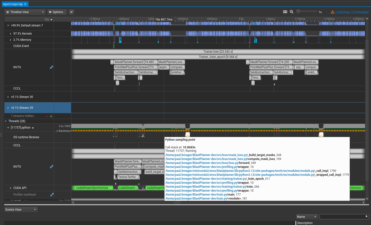
Using the Python call stack samples, you can hover over the sync and see exactly what line triggered it. For me it was:
n_strokes_per = (group_idx_sorted.max(dim=-1).values + 1).clamp(min=0)  # (B,)
max_n = max(int(n_strokes_per.max().item()), 1)
The .item() call reads a GPU tensor value back to the CPU, which forces a sync. It makes sense: to know what n_strokes_per.max() is, the GPU has to finish computing it.
Sometimes you can remove these syncs, sometimes you can’t. In this case, I was able to restructure the preprocessing and collation logic so that max_n becomes a constant known ahead of time:
max_n = n_masks
And the performance improvement is …. nothing.
Doing something genuinely clever and getting zero speedup out of it is part of the process. But looking at the new trace, build_target_masks now flies through almost invisibly. Progress.
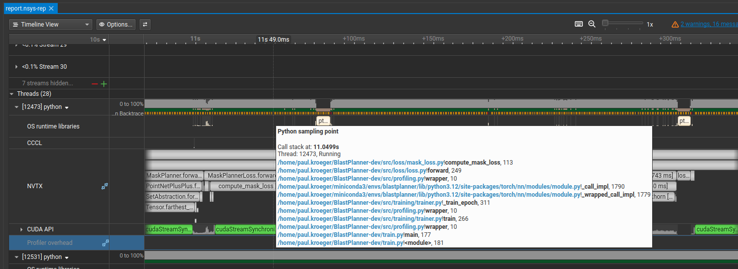
There’s still a large sync in compute_mask_loss. Hovering over the Python call stack at that point reveals:
if not stroke_valid.any():
    return pred_mask_logits.sum() * 0.0  # keep grad graph alive, zero
The CPU needs to evaluate that condition, which means it has to wait for stroke_valid.any() to come back from the GPU. This turned out to be a data quality guard that only existed because of some messy training data. Cleaning the dataset and moving the check to preprocessing removed it from the hot path entirely.
I ran into variations of this probably 4 or 5 times. I’ll spare you the details of a codebase you don’t have access to. The bottom line is that the hot path is now mostly free of unnecessary syncs, and we’re at 160 samples/second (up from 140, about 15%).
Here’s what the final sync picture looks like:
For those curious: the first (large) sync is from a point encoder in the forward pass whose output is needed before the rest of the network can condition on it, so that one’s unavoidable. The second comes from computing a bipartite matching in the loss function. The third is the final sync at the end of the epoch when we wait for the last batch to complete.
Compiling your model
torch.compile() uses TorchDynamo to trace through your model and passes the result to the Inductor backend, which compiles it down to optimized GPU code via Triton. In practice, the main win is kernel fusion: instead of launching a separate CUDA kernel for every individual operation (add, normalize, activate, …), the compiler merges them into fewer, larger kernels. This reduces kernel launch overhead and can improve memory access patterns significantly.
It’s a one-line change:
model = torch.compile(model)
loss_fn = torch.compile(loss_fn)
The first few iterations will be slower while the compiler traces the graph. After warmup, you should see a consistent improvement. If your model uses heavily dynamic shapes (variable sequence lengths, ragged batches, etc.), compile can be less effective or occasionally cause issues. I like this user guide for getting more out of it.
This takes us from 160 to 170 samples/second.
Mixed precision
torch.autocast runs compute-heavy operations like matrix multiplications and convolutions in FP16 or BF16, while keeping numerically sensitive operations in FP32. NVIDIA GPUs have dedicated Tensor Core hardware for FP16/BF16 matmuls, and the throughput difference is significant.
with torch.autocast(device_type='cuda', dtype=torch.bfloat16):
    output = model(pc)
    loss, breakdown = loss_fn(output, batch, epoch=epoch)
If you use FP16 rather than BF16, you’ll also want a GradScaler to handle gradient underflow. BF16 has the same exponent range as FP32 (8 bits vs 5 in FP16) so underflow is much less of an issue, but BF16 Tensor Cores require Ampere or newer hardware.
This brings us from 170 to 240 samples/second. Pretty huge.
A note on loss functions
I want to mention something that was actually the first change I made and the single biggest improvement overall, even though it’s specific enough that it probably won’t apply directly to your code.
The original system used Hungarian matching to compute a bipartite assignment in the loss. Hungarian matching finds the exact optimal assignment in O(n³), and it’s fundamentally sequential, making it very hard to parallelize on a GPU. People have tried GPU implementations (here’s one) but it’s a difficult problem that typically requires custom CUDA kernels.
I replaced it with Sinkhorn distance, which approximates the optimal transport problem via iterative matrix scaling. The whole thing is batched matrix operations, so it runs efficiently on the GPU without any custom kernels. For my use case it was essentially a drop-in replacement and cut the forward pass through the loss by about 60%.
The reason I put this at the end rather than the beginning is that it won’t transfer directly to most problems. But there’s a broader point worth keeping in mind: it’s often justified to trade a theoretically precise loss for a faster, slightly less precise one. Faster iterations compound. More experiments in the same wall-clock time often matters more than the exactness of the loss formulation.
Where we ended up
A few hours of profiling, identifying bottlenecks, and patching them got us from 65 to 240 samples/second, roughly a 3.7x improvement. The changes were:
| Change | Samples/s |
|---|---|
| Baseline | 65 |
| DataLoader (workers, pin_memory, non_blocking) | 75 |
| Replace custom FPS with torch_cluster | 140 |
| Remove unnecessary GPU syncs | 160 |
| torch.compile | 170 |
| Mixed precision | 240 |
The main takeaway is that optimization doesn’t have to wait until research is done. Treating it as part of the process cuts experiment time and cost, and that directly speeds up iteration. Hardware constraints are also worth thinking about early. A theoretically elegant model or loss that’s slow to compute will often lose out to a simpler, faster one in practice.
Next steps
You’d be surprised what a Karpathy-style autoResearch system can squeeze out of this pipeline. More on that in a future post.
References
- torch.compile user guide
- Speed up PyTorch training with Nsight
- Nsight Systems systematic optimization
- CUDA programming guide
If this kind of work sounds interesting, please to reach out.