I’ve always had a lurking interest in reinforcement learning, but only recently did I find the time to revisit some of the basics. Part of “going back to the roots” was looking at the first truly groundbreaking deep reinforcement learning papers. Among these, the ones that showed deep RL agents could play Atari games. Back in 2015, this was so astonishing that it even made mainstream news.
Besides the fact that the original papers are freely available (this list is a great place to start), there’s no shortage of tutorials, blog posts, and lecture notes explaining how deep RL works. Still, I thought it would be fun to write one more “from scratch” implementation—partly for my own learning and partly because I think I can add a few fresh angles that others might find useful. Feedback is, of course, very welcome.
If you’re mostly here for the code, feel free to jump ahead to the implementation section. The first couple of sections are just a recap of the key ideas we’ll need.
The Problem
Imagine you’re as terrible at arcade games as I am. You still want to impress your friends with a massive high score, so you decide to train a computer to play for you. Ideally, you want the computer to have the same inputs that you do, i.e. just the raw screen pixels.
Fortunately, Mnih et al. solved just this problem in their influential 2015 paper, Playing Atari with Deep Reinforcement Learning. Their big idea was simple but powerful: feed the current game frame into a neural network, and have it predict which action is best.
Of course, the real question is: how does the network know which action is good in the first place? That’s where reinforcement learning comes in. We’ll recap just enough theory to make sense of this before diving into the machine deep machine learning version.
A (very) brief Introduction to Reinforcement Learning
Reinforcement learning is about training an agent to make decisions by interacting with an environment. At each step, the agent sees a state (s), chooses an action (a), receives a reward (r), and transitions to a new state (s’). This loop is often formalized as a Markov Decision Process.
The agent’s goal is to maximize the expected return, which is the discounted sum of future rewards:
$$ G_t = \sum_{k=0}^\infty \gamma^k r_{t+k+1} $$
where $0 \leq \gamma < 1$ is the discount factor that balances immediate versus long-term rewards. The agent’s behavior is governed by a policy $\pi$, which tells us how actions are chosen in each state. Formally, $\pi(a \mid s)$ is the probability of taking action $a$ in state $s$.
To evaluate policies, we define value functions. The state-value function measures the expected return from state $s$:
$$ V^\pi(s) = \mathbb{E}_\pi \left[ G_t \mid S_t = s \right] $$
The action-value function (or Q-function) measures the expected return from taking action $a$ in state $s$:
$$ Q^\pi(s,a) = \mathbb{E}_\pi \big[ G_t \mid S_t = s, A_t = a \big] $$
The optimal Q-function satisfies the Bellman optimality equation:
$$ Q^{\ast}(s,a) = \mathbb{E}\left[ r + \gamma \max_{a’} Q^*(s’,a’) \mid s,a \right] $$
Interestingly, (due to the uniqueness of fixed points) the optimal Q-function is unique. That means that for any Q-function $Q$ satisfing the above equation, we have $Q = Q^{\ast}$
Building open this result, Q-learning is an algorithm that directly approximates the optimal Q-function. It updates estimates using:
$$ Q(s,a) \leftarrow Q(s,a) + \alpha \left[ r + \gamma \max_{a’} Q(s’,a’) - Q(s,a) \right] $$
Here $\alpha$ is the learning rate, and the term in brackets is the temporal-difference error. Once trained, the agent acts greedily:
$$ \pi(s) = \arg\max_a Q(s,a) $$
Deep Q-Learning
Now let’s return to the Atari problem. Using the classical RL formulation, the idea behind deep Q-learning (DQN) is actually quite straightforward. Suppose our environment has $n_a$ possible actions. We take a neural network, feed it the current screen frame as input, and let it output an $n_a$-dimensional vector. For a given state $s$, the $i$-th entry corresponds to the Q-value $Q(s, a_i)$. By taking the argmax over this vector, we select the action the network thinks is best.
During training, we execute that action in the environment, observe a reward $r$ and a next state $s’$, and then update the network to reduce the temporal-difference error defined by the Bellman equation. Concretely, the loss is based on the difference between the predicted Q-value and the target value. To make this stable in practice, the authors introduce a target network, a copy of the Q-network whose parameters are held fixed for a while and only updated periodically. This trick prevents the network from chasing its own moving targets and was one of the key innovations of the original DQN paper.
$$ y = r + \gamma \max_{a’} Q(s’,a’; \theta^-) $$
$$ L(\theta) = \big( Q(s,a;\theta) - y \big)^2 $$
Here $\theta$ are the network parameters, and $\theta^-$ are the parameters of the target network.
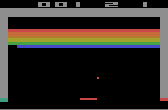
While there are many additional details needed to make this work well in practice (we’ll get to those later), there’s one conceptual issue to address right away: using only a single frame as input often makes the state of Atari games ambiguous. For example, looking at the screenshot below, you can’t immediately tell which way the ball is moving.
Humans solve this by using information about previously seen frames to infer the direction in which the ball is moving. But our model, in its current form, has no explicit memory of past states. To give it a similar capability, the original DQN stacked the last four frames together as input to their network. This way, the network can infer motion and dynamics across time. (Later work also experimented with adding recurrent networks like LSTMs to give agents true memory, but we’ll stick to the frame-stacking approach here.)
Here’s a draft for your new section, written in the same casual/approachable tone as the rest of your blog. I’ve kept it light but clear, with references to the classic papers you linked:
Problems With Deep Q-Learning
While the idea decribed above already yields interesting results, over the years people have realized issues with vanially DQN and come up with many interesting improvements. I picked two of them that I really like and implemented them here as well to improve performance of our agent.
The Role of Replay Memory (and Why Prioritization Helps )
In vanilla Q-learning, every new step you take in the environment is immediately used for a training update. That sounds fine, but it creates two problems: (1) consecutive frames in a game are highly correlated, which means your network is basically being trained on near-duplicate data, introducing high bias, and (2) once you move on from a state, that experience is gone forever—an inefficient use of data.
DQN addresses this by introducing replay memory (also called an experience buffer). Every time you interact with the environment, you store the transition tuple ((s, a, r, s’)) in the buffer. Then, instead of training only on the latest sample, you periodically draw random mini-batches of transitions from this buffer and use them for training updates. This does two things: it breaks correlations between consecutive frames (since your batches are now mixed) and it lets the agent “revisit” old experiences many times, making learning much more data-efficient.
A typical training loop looks something like this:
Interact with the environment, store each ((s,a,r,s’)) in the replay memory.
Once the buffer has enough samples, start training.
For each update step:
- Sample a mini-batch of transitions uniformly at random from the buffer.
- Compute the TD target and loss.
- Backpropagate to update the Q-network.
Repeat: keep collecting more transitions and keep sampling from the buffer.
How much new data you collect versus how many training updates you do per environment step is implementation-dependent, but can have a surprisingly large impact on performance. Some implementations update the network every single step, others do several updates per step, and others only update every few steps. The specifics often depend on how costly it is to sample data from the environment. Similarly, the buffer size, batch size, and how long experiences “live” in the buffer are all design choices that affect stability and data efficiency.
Replay memory gives us a way to recycle experiences and break correlations between consecutive frames. But once you think about it, sampling uniformly at random from the buffer is a bit wasteful. Some transitions are just not that useful for learning, while others are far more informative.
For example, imagine you’re training Breakout and the agent has already mastered moving the paddle when the ball comes straight down. Those transitions will appear again and again in the buffer, but they don’t teach the agent anything new. On the other hand, rare or surprising events—like missing the ball in an unexpected way—might produce a large temporal-difference (TD) error, meaning the agent’s prediction was very wrong. Intuitively, we want the agent to spend more time improving in those tougher situations.
This insight led to Prioritized Experience Replay (Schaul et al., 2015). The idea is simple: instead of sampling uniformly, we sample experiences with probability proportional to how “important” they are, where importance is measured by the TD error. The probability $p_i$ of sampling transition $i$ from memory is given by:
[ p_i = \frac{|\delta_i|^\alpha}{\sum_j |\delta_j|^\alpha} ]
Here (\delta_i) is the TD error of transition (i), and (\alpha \geq 0) controls how much prioritization we use. If (\alpha = 0), this reduces to uniform sampling. Larger (\alpha) makes the buffer focus more on high-error samples.
There’s a catch though: biased sampling changes the distribution of training data, which can in turn bias the Q-value estimates. To fix this, Prioritized Experience Replay introduces importance-sampling weights during training. The loss coming from sample $i$ has to be rescaled using the weight $w_i$:
[ w_i = \Big( \frac{1}{N \cdot p_i} \Big)^\beta ]
where (N) is the buffer size and (\beta) gradually anneals from a small value toward 1 over training. These weights are applied to the loss, so that transitions sampled more frequently don’t skew learning too much.
In practice, the recipe looks like this:
- Store transitions ((s,a,r,s’)) in replay memory with an initial priority (often the max seen so far so that new transitions get used at least once).
- When sampling a batch, draw transitions according to (p_i).
- Compute the TD errors for that batch.
- Update both the Q-network and the priorities in the replay buffer.
This way, the buffer automatically shifts focus toward the experiences where the agent is currently making the biggest mistakes, leading to faster and more efficient learning.
We will later see how to implement this idea, but there a lot of interesting details to this approach that we didn’t cover. For example, there is quite some nuance required when picking the factors $\alpha$ and $\beta$. For these details you should definitely take a look at the original paper.
Double Q-Learning (and Why It Fixes Overestimation Bias )
Another problem with the original DQN is something called overestimation bias. The issue comes from the target used in vanilla Q-learning:
[ y = r + \gamma \max_{a’} Q(s’, a’; \theta) ]
Here the same network (with parameters (\theta)) is used both to select the action (via the max) and to evaluate it. That might not sound too bad, but if the Q-values are noisy—which they inevitably are during training—the max tends to systematically overshoot. In other words, the agent consistently thinks actions are better than they really are. This can make training unstable and sometimes push the agent toward poor strategies.
van Hasselt et al., 2015 solve this problem by introducing Double Q-Learning. The idea is to decouple the action selection step from the action evaluation step. Instead of using one network for both, we use two:
- The main (online) network with parameters (\theta) is used to select the action with the highest estimated value.
- The target network with parameters (\theta^-) is used to evaluate that chosen action.
Formally, the target becomes:
[ y = r + \gamma Q\Big(s’, \arg\max_{a’} Q(s’,a’;\theta); \theta^- \Big) ]
Notice how the (\arg\max) comes from the online network, while the Q-value used in the target comes from the target network. This small change dramatically reduces the bias introduced by noisy max estimates.
In practice, Double DQN looks almost identical to vanilla DQN—the training loop is the same, you’re just swapping out the way you compute the target. For comparison here is the vanialla DQN target again:
[ y = r + \gamma \max_{a’} Q(s’,a’; \theta^-) ]
Again, for a sound argument of why this works, please check out the paper!
Implementation
Now, finally, we are ready to dive into the implementation.